z <- read.table("Mickelia_nicot_datos.csv", header=TRUE, sep=",")
str(z)
## 'data.frame':    12 obs. of  9 variables:
##  $ Habit                 : chr  "terrestrial_1" "Terrestrial_2" "Terrestrial_3" "Terrestrial_4" ...
##  $ number_leaves_sampled : int  2 2 2 2 2 2 2 2 2 2 ...
##  $ Pinnae_numb           : int  1 3 3 3 5 5 5 3 5 5 ...
##  $ Leaf_size_cm          : num  13 18 21 18 23 23.4 22.7 17.5 15 16.2 ...
##  $ Petiole_size          : num  4.5 6 8.5 5.8 11 11 11 8 7.8 8 ...
##  $ Pinnae_size_cm        : num  5 5.5 6 6 8 8 7.6 8 5 6 ...
##  $ laminae_widht_cm      : num  10 10 9.7 9 18 17 17.7 17.5 8 8 ...
##  $ pinnae_withd_cm       : num  3.3 4 3.5 4 6 5.5 4.8 6 3 2.5 ...
##  $ Petiole_scales_size_cm: num  0.4 0.35 0.4 0.3 0.25 0.28 0.33 0.35 0.2 0.18 ...
summary(z)
##     Habit           number_leaves_sampled  Pinnae_numb     Leaf_size_cm
##  Length:12          Min.   :2             Min.   :1.000   Min.   :13.00
##  Class :character   1st Qu.:2             1st Qu.:3.000   1st Qu.:15.30
##  Mode  :character   Median :2             Median :3.000   Median :17.75
##                     Mean   :2             Mean   :3.667   Mean   :18.17
##                     3rd Qu.:2             3rd Qu.:5.000   3rd Qu.:21.43
##                     Max.   :2             Max.   :5.000   Max.   :23.40
##   Petiole_size    Pinnae_size_cm  laminae_widht_cm pinnae_withd_cm
##  Min.   : 4.500   Min.   :5.000   Min.   : 8.00    Min.   :2.500
##  1st Qu.: 6.750   1st Qu.:5.000   1st Qu.: 8.75    1st Qu.:3.150
##  Median : 7.900   Median :6.000   Median : 9.85    Median :3.750
##  Mean   : 7.983   Mean   :6.258   Mean   :11.82    Mean   :4.067
##  3rd Qu.: 9.125   3rd Qu.:7.700   3rd Qu.:17.12    3rd Qu.:4.975
##  Max.   :11.000   Max.   :8.000   Max.   :18.00    Max.   :6.000
##  Petiole_scales_size_cm
##  Min.   :0.1800
##  1st Qu.:0.2075
##  Median :0.2900
##  Mean   :0.2867
##  3rd Qu.:0.3500
##  Max.   :0.4000
library(ggplot2)
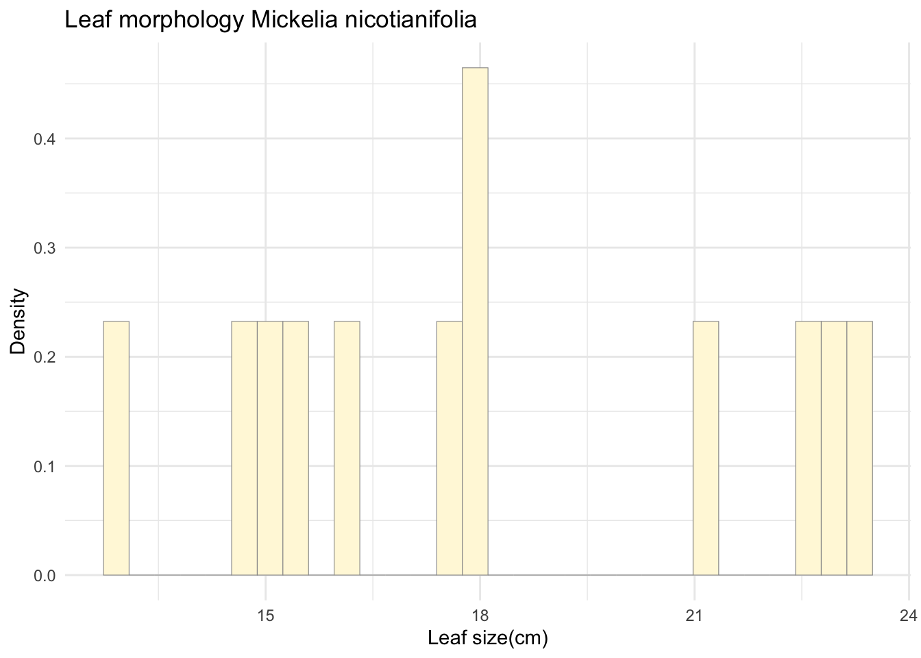
p1 <- ggplot(data=z, aes(x=Leaf_size_cm, y=..density..)) +
geom_histogram(color="grey60", fill="cornsilk", size=0.2) +
labs(title="Leaf morphology Mickelia nicotianifolia",
x="Leaf size(cm)",
y="Density") +
theme_minimal()
## Warning: Using `size` aesthetic for lines was deprecated in ggplot2 3.4.0.
## ℹ Please use `linewidth` instead.
## This warning is displayed once every 8 hours.
## Call `lifecycle::last_lifecycle_warnings()` to see where this
## warning was generated.
print(p1)
## Warning: The dot-dot notation (`..density..`) was deprecated in ggplot2
## 3.4.0.
## ℹ Please use `after_stat(density)` instead.
## This warning is displayed once every 8 hours.
## Call `lifecycle::last_lifecycle_warnings()` to see where this
## warning was generated.
## `stat_bin()` using `bins = 30`. Pick better value with `binwidth`.
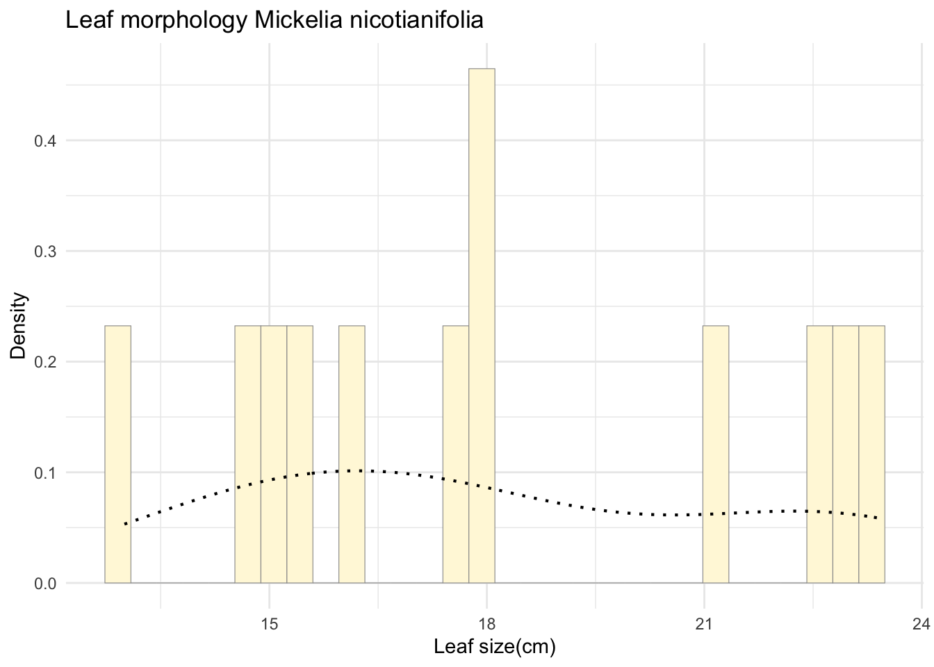
p1 <-  p1 +  geom_density(linetype="dotted",size=0.75)
print(p1)
## `stat_bin()` using `bins = 30`. Pick better value with `binwidth`.
library(MASS)
##
## Attaching package: 'MASS'
## The following object is masked from 'package:dplyr':
##
##     select
normPars <- fitdistr(z$Leaf_size_cm, "normal")

print(normPars)
##       mean          sd
##   18.1666667    3.4084046
##  ( 0.9839217) ( 0.6957377)
str(normPars)
## List of 5
##  $ estimate: Named num [1:2] 18.17 3.41
##   ..- attr(*, "names")= chr [1:2] "mean" "sd"
##  $ sd      : Named num [1:2] 0.984 0.696
##   ..- attr(*, "names")= chr [1:2] "mean" "sd"
##  $ vcov    : num [1:2, 1:2] 0.968 0 0 0.484
##   ..- attr(*, "dimnames")=List of 2
##   .. ..$ : chr [1:2] "mean" "sd"
##   .. ..$ : chr [1:2] "mean" "sd"
##  $ n       : int 12
##  $ loglik  : num -31.7
##  - attr(*, "class")= chr "fitdistr"
mean_estimate <- normPars$estimate["mean"]
print(mean_estimate)
##     mean
## 18.16667
meanML <- normPars$estimate["mean"]
sdML <- normPars$estimate["sd"]
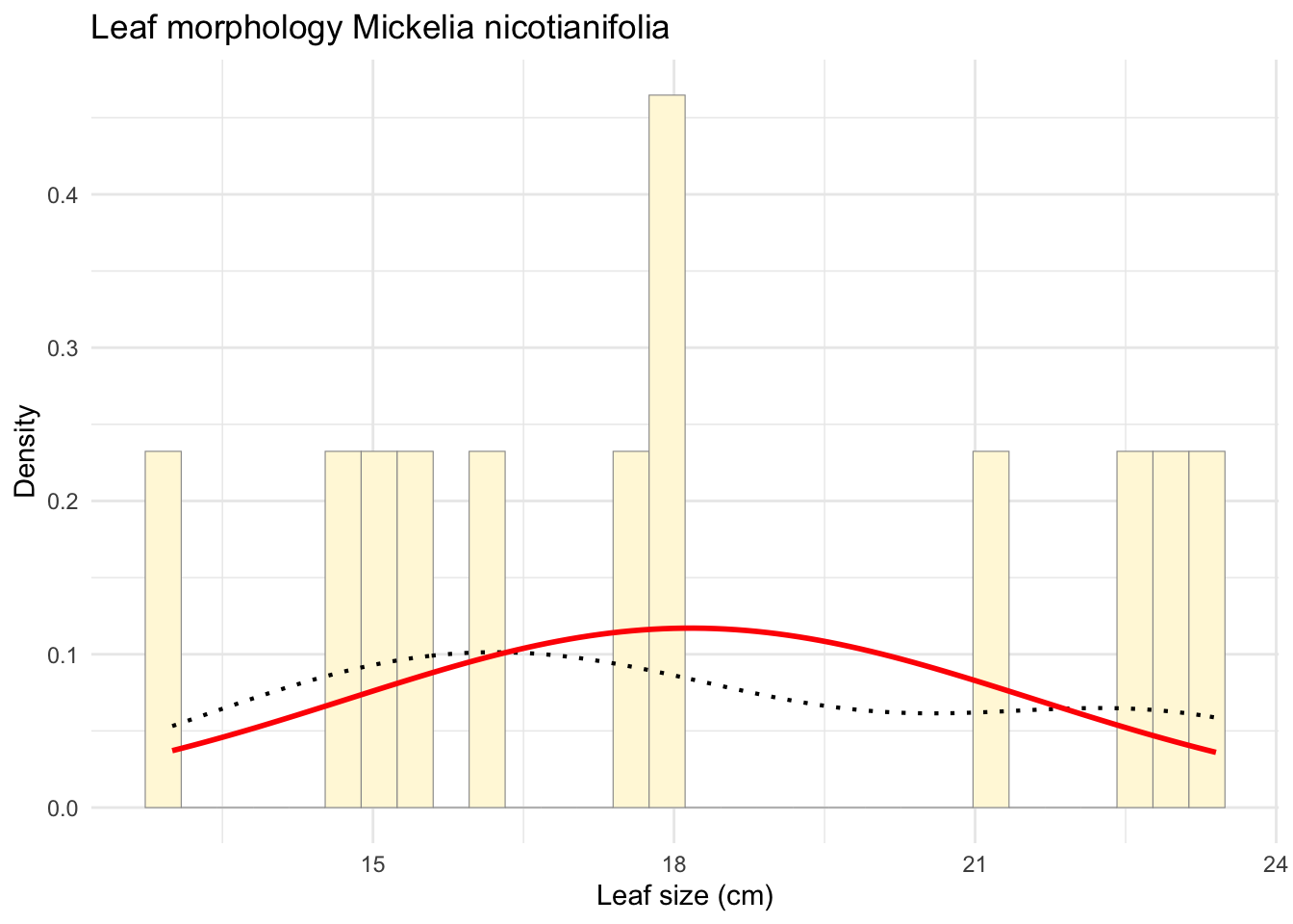
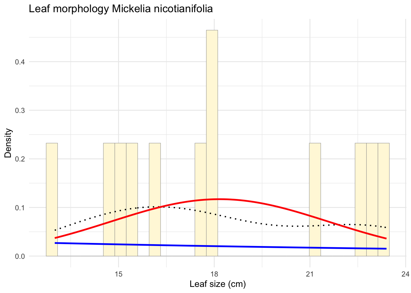
p1 <- ggplot(data=z, aes(x=Leaf_size_cm)) +
geom_histogram(aes(y = ..density..), color="grey60", fill="cornsilk",
size=0.2, bins=30) + # Usar density aquí
labs(title="Leaf morphology Mickelia nicotianifolia",
x="Leaf size (cm)",
y="Density") +
theme_minimal() +
geom_density(aes(y = ..density..), linetype="dotted", size=0.75) +
stat_function(fun = dnorm,
args = list(mean = meanML, sd = sdML),
colour = "red",
size = 1)
print(p1)
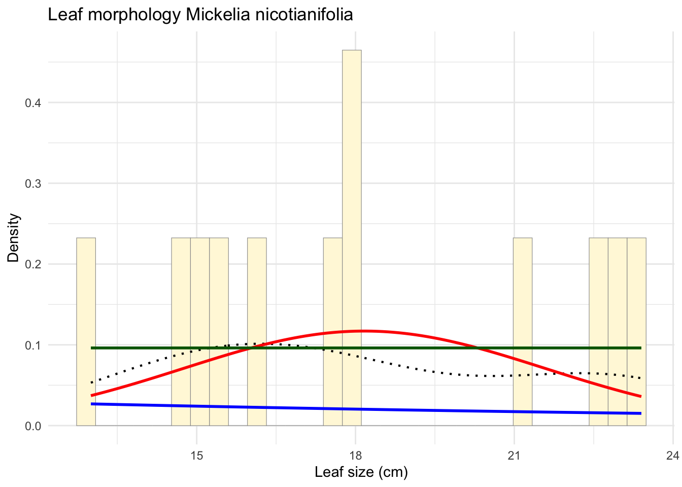
expoPars <- fitdistr(z$Leaf_size_cm, "exponential")
rateML <- expoPars$estimate["rate"]

xval <- seq(0, max(z$Leaf_size_cm, na.rm = TRUE), length.out = length(z$Leaf_size_cm))

stat2 <- stat_function(fun = dexp,
                       args = list(rate = rateML),
                       colour = "blue",
                       size = 1)

p_combined <- p1 + stat2
print(p_combined)
min_val <- min(z$Leaf_size_cm)
max_val <- max(z$Leaf_size_cm)

stat3 <- stat_function(fun = dunif,
                       args = list(min = min_val, max = max_val),
                       colour = "darkgreen",
                       size = 1)

p_final <- p_combined + stat3
print(p_final)
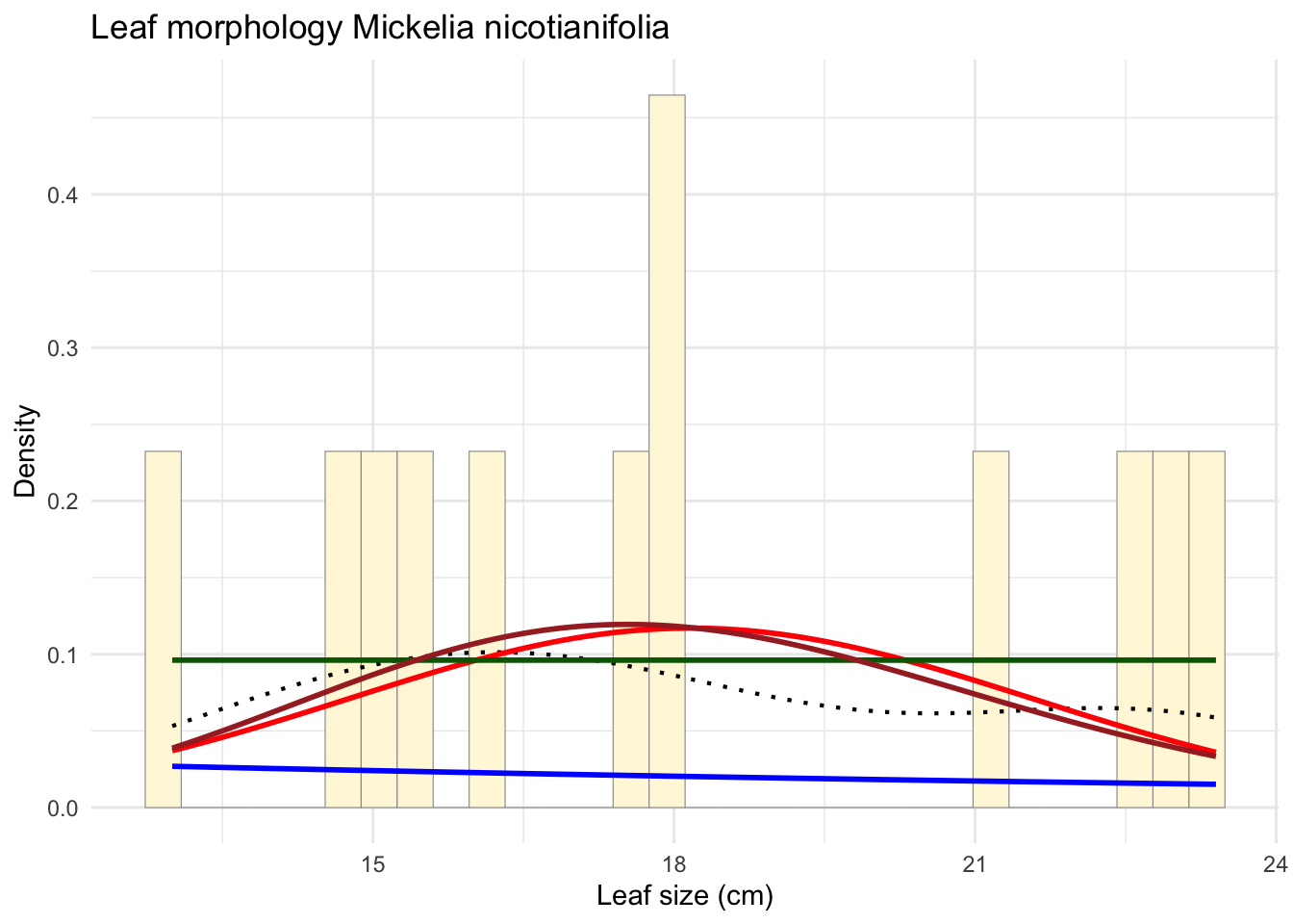
gammaPars <- fitdistr(z$Leaf_size_cm, "gamma")
shapeML <- gammaPars$estimate["shape"]
rateML <- gammaPars$estimate["rate"]

stat4 <- stat_function(fun = dgamma,
                       args = list(shape = shapeML, rate = rateML),
                       colour = "brown",
                       size = 1)

p_final <- p_final + stat4
print(p_final)
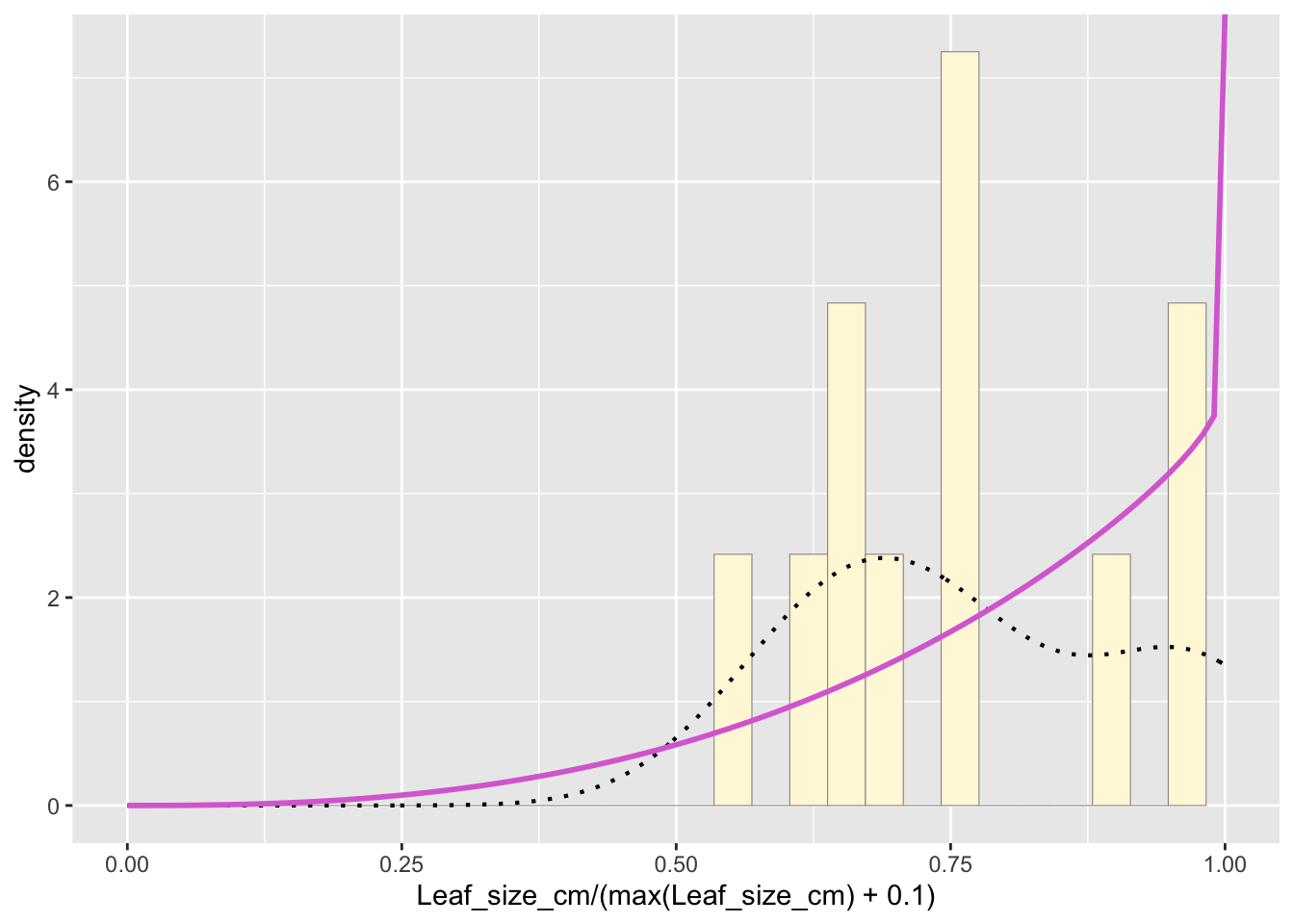
pSpecial <- ggplot(data=z,
                   aes(x=Leaf_size_cm/(max(Leaf_size_cm) + 0.1))) +
  geom_histogram(aes(y = ..density..), color="grey60", fill="cornsilk", size=0.2, bins=30) +
  xlim(c(0,1)) +
  geom_density(size=0.75, linetype="dotted")

betaPars <- fitdistr(x=z$Leaf_size_cm/max(z$Leaf_size_cm + 0.1), start=list(shape1=1, shape2=2), "beta")
## Warning in densfun(x, parm[1], parm[2], ...): NaNs produced
## Warning in densfun(x, parm[1], parm[2], ...): NaNs produced
## Warning in densfun(x, parm[1], parm[2], ...): NaNs produced
## Warning in densfun(x, parm[1], parm[2], ...): NaNs produced
shape1ML <- betaPars$estimate["shape1"]
shape2ML <- betaPars$estimate["shape2"]

statSpecial <- stat_function(fun = dbeta,
                             args = list(shape1=shape1ML, shape2=shape2ML),
                             colour = "orchid",
                             size = 1)
pSpecial + statSpecial
## Warning: Removed 2 rows containing missing values or values outside the
## scale range (`geom_bar()`).